
30 Percent Better Accuracy Without Dropping Half the Dataset
It Improved the Moment I Looked at Why Data Was Missing.


It is always good to have all in place and clean. The reality is different, and our datasets are not complete, and there are some gaps in them.
There is a Broken Windows Theory, which states that broken windows and similar signs for a prolonged period lead to increased levels of crime. Instead of a high rate of crime, unclear and partial data can introduce overall chaos in an organization, and it affects all other aspects of the business and is related to the whole structure of the company, affecting all kinds of departments, not only data.
As data analysts, we work with what we have, and getting a proper strategy for handling missing data is the crucial step of analysis, as, according to the surveys, data analysts spend around 70% of their time in data cleaning.
What is missing?
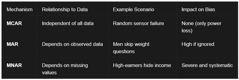
There are 3 main types of missing data:
Missing Completely at Random (MCAR):
Data is classified as Missing Completely at Random (MCAR) if the probability of a value missing is entirely independent of any observed or unobserved variables in the dataset.
When data is MCAR, the observed records can be considered a simple random sample of the full dataset. While the loss of data reduces the population to analyze and the statistical power, it does not introduce bias into parameter estimates.
In such cases, the analysis of remaining data, a complete case analysis, provides an unbiased estimate of the truth.
2. Missing at Random (MAR):
The term Missing at Random (MAR) implies that the missingness is systematically related to observed data but not to the missing values themselves.
The critical implication of MAR is that the missingness can be explained by other variables in the dataset. By using observed variables like sex or age to model the missingness, analysts can employ techniques such as multiple imputation or weighted estimation to produce unbiased results.
If we ignore these observed factors, a complete case analysis will become severely biased.
3. Missing Not at Random (MNAR):
Missing Not at Random (MNAR) is the most problematic, where the probability of missingness is related to the unobserved value itself.
A common example occurs in financial surveys: individuals with either extremely high or extremely low incomes may be more likely to refuse to disclose their earnings. Similarly, patients with the most severe symptoms in a clinical trial might be the ones most likely to drop out because they are too ill to attend follow-up appointments.
MNAR data introduces significant bias that is difficult to address without external validation or domain expertise. If you ignore MNAR mechanisms, this will lead to invalid conclusions.
What we can do with missing values?
Common Strategies for Handling Missing Data:
Which should you choose? It depends on three factors:
How much data is missing? A few rows? Drop them. A third of your dataset? Probably, Fill.
Why is it missing? Random gaps are safer to fill. Systematic missingness (like high earners refusing to share their salary) requires careful thought.
What is your goal? Exploratory analysis can tolerate more aggressive fill.
Another approach is to understand the missing data type and patterns.
This code will help us visualize the missing data.
import matplotlib.pyplot as plt
import missingno as msno
# Visualize missing data
msno.matrix(df)
plt.show()msno.heatmap(df)
plt.show()If you see some patterns and data missing not at random, separate it and investigate the reason why it happened.
Run Little’s MCAR test to identify the nature of missing values.
from statsmodels.imputation import mice# Run Little’s MCAR Test
imputer = mice.MICEData(df)
mcar_test_result = imputer.mcar_test()
print(mcar_test_result)P > 0.05 ?
↳ If answer is No, this data is Missing at Random (MAR).
↳ If answer is Yes, this data is Missing at Completely at Random (MCAR).
Here are the recommendations:
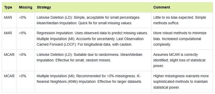
There is no one-size-fits-all solution, but here are the most popular approaches:
1. Deletion:
Listwise Deletion: Remove any row with missing data. Simple, but you lose information and can bias results if data is not MCAR.
Pairwise Deletion: Use all available data for each calculation. Keeps more data but can lead to inconsistent sample sizes.
2. Imputation:
Mean/Median/Mode Imputation: Fill gaps with the average, median, or most common value. This is easy but can distort variability and relationships.
Multiple Imputation: Create several versions of the dataset with different plausible values, then combine results. It is more accurate but more complex.
Machine Learning Imputation: Use algorithms like k-Nearest Neighbors or Random Forests to predict missing values.
3. Special Handling:
Flag or Label: Mark missing values with a special code (“Unknown,” “N/A”) so you can track them.
Fill Forward/Backward: For time series, fill gaps with the previous or next value.
Custom Logic: Use business rules or domain knowledge to decide what to do.
4. Advanced Techniques:
Interpolation for sequential data or machine learning-based imputation for complex patterns.
If data is MCAR: Simple deletion or imputation is fine.
If data is MAR: Use multiple imputation, regression imputation, or advanced methods.
If data is MNAR: Run a modeling and sensitivity analysis, and be cautious about conclusions.
Debates and Trade-Offs: What is the Best Approach?
Deletion is simple but risky. If your data is MCAR and you don’t lose too many rows, it is fine. But if missingness is not random, you can bias your results.
Imputation preserves data but can introduce bias. Simple methods (mean, median) are quick but can flatten your data. Advanced methods (multiple imputation, machine learning) are better but require more work and expertise.
Multiple Imputation is the gold standard for MAR. It accounts for uncertainty and gives more reliable results, but it is computationally intensive.
For MNAR, no method is perfect. You may need to model the missingness itself or run sensitivity analyses.
When you use imputation, make sure to plot the distribution before and after imputation. This is an important step, as some methods might change the data distribution and affect a following analysis.
Application in SQL:
SQL is best for quick filtering and basic imputation in structured datasets.
Use SQL when you need speed and simplicity, but be cautious about deleting too many rows with missing data, as it might shrink your dataset too much and bias the results.
NULL vs. Empty: What is the Difference?
In SQL, NULL means “no value”, and the data is missing or unknown. An empty string (“”) means the value exists but is blank. For numbers, 0 is a value, not missing. This distinction matters for queries and calculations.
Example:
NULL in a column: The value was not provided.
‘’ (empty string): The value was provided, but it is blank.
0: The value is zero, not missing.
SQL operates on three-valued logic:
True,
False,
Unknown (NULL).
This creates unique behaviors in queries:
For example, a standard comparison like WHERE column = 5 will exclude rows where the column is NULL, because the database cannot confirm if an unknown value equals five. To capture these rows, utilize the specific operators IS NULL and IS NOT NULL.
Aggregate functions such as SUM(), AVG(), and COUNT() typically ignore NULL values. While this is the desired behavior, it can lead to discrepancies if you expect NULL to be treated as a zero.
In a scenario where 100 orders are placed but only 80 have a recorded OrderAmount, AVG(OrderAmount) will calculate the average of those 80, potentially overestimating the typical order size if the missing values were likely to be small.
Core SQL Functions for NULL Transformation:
COALESCE(): This function takes multiple arguments and returns the first non-null value in the list. It is frequently used to establish fallback hierarchies. For instance, a customer profile query might use COALESCE(MobilePhone, WorkPhone, Email, ‘Unknown’) to ensure a contact method is always displayed.
ISNULL() / IFNULL(): These are database-specific variations (SQL Server and MySQL, respectively) that take two arguments and replace a NULL with a specified default. While less flexible than COALESCE, they are preferred for simple, high-performance substitutions.
NULLIF(): This function performs the opposite task: it returns NULL if two expressions are equal. This is vital for cleaning bad data, such as converting an empty string (‘’) or a placeholder like 0 into a true NULL so it can be handled by standard missingness logic later in the pipeline. In MySQL and PostgreSQL empty text values are not null by default and should be replaced before by using NULLIF.
CASE Statements: For complex business logic, the CASE expression allows for conditional imputation. An analyst might use CASE WHEN Quantity IS NULL THEN 0 ELSE Quantity END to ensure numerical measures are safe for arithmetic.
Handling NULLs in Aggregations and Joins:
Aggregations: Functions like SUM(), AVG(), MIN(), and MAX() ignore NULLs. COUNT(*) counts all rows; COUNT(column) counts only non-NULL values.
Joins: OUTER JOINs can introduce NULLs when there is no match.
Application in Python:
Python is ideal for complex datasets that require advanced imputation and automation. Use Python when you need fine control over imputation methods or when dealing with unstructured or nested data.
Key Methods
Deletion:
dropna(): This method can be configured to drop rows or columns based on the extent of their missingness. Using the threshold parameter, an analyst can drop columns only if they have fewer than a certain number of non-missing values and preserve columns that are mostly complete.
# Drop rows with any NaN values
df_cleaned = df.dropna(axis=0)

# Drop rows with any NaN values from specific column
df = df.dropna(subset=[’City’])Filling:
fillna(): This method provides the tools for single imputation. Beyond simple constants, it can implement statistical imputation, such as filling missing ages with the median value of the column. It also supports “forward fill” (ffill) and “backward fill” (bfill), which are indispensable in time-series data where the last observed value is assumed to remain constant until a new read occurs.
df[’colname’].replace({’D’: ‘F’, ‘N’: ‘M’}) # replace one value with other

df[’columns_mame’] = df[’columns_mame’].fillna(0) # replace with 0

df.Description = df.Description.replace(np.nan, ‘No Description’) # fill with default value

df.fillna(df.mean()) # fill with mean

df.fillna(df.median())# fill with median

df.fillna(df.mode())# fill with mode

df.ffil # propagate the last valid observation to next valid

df.fillna(method = bfill) # fill with next value, axis = 1 for row

df.fillna(method = PAD) # fill with previous value
Interpolation:
Interpolation is an estimation technique that fills gaps by looking at the trend of surrounding data points. Unlike fillna(), which uses a static value, interpolate() is dynamic and adapts to the data’s pattern.
Linear Interpolation: This is the default method, creating a straight-line transition between two known points. For a simple sequence like [1, NaN, 3], linear interpolation correctly guesses 2.0.
Time-Based Interpolation: In datasets with a time-series index, this method accounts for the actual time elapsed between observations. If data points are recorded on January 1st and January 4th, the gap is treated differently than a gap between January 1st and 2nd.
Polynomial and Spline Interpolation: For data representing natural processes, such as a plant growth or a car acceleration, straight lines are unrealistic. Polynomial interpolation uses a curve to fill gaps, providing a more accurate estimate for accelerating or decelerating trends.
import pandas as pd
import numpy as np


# Linear Interpolation
df[”linear”] = df[”value”].interpolate()

# Polynomial Interpolation
df[”poly2”] = df[”value”].interpolate(method=”polynomial”, order=2)

# Spline Interpolation
df[”spline2”] = df[”value”].interpolate(method=”spline”, order=2)

# Time-Based Interpolation
ts_time = ts.interpolate(method=”time”)
Advanced imputation methods:
For scientific or financial analysis, simple imputation is criticized for artificially reducing the variance of the data and potentially masking real-world uncertainty. Advanced Python libraries enable more robust techniques:
Multiple Imputation by Chained Equations (MICE): This process involves creating several “complete” datasets by iteratively modeling each missing variable as a function of the others. By analyzing these multiple datasets and pooling the results, analysts can account for the uncertainty inherent in the imputation process, resulting in more accurate standard errors and confidence intervals.
k-Nearest Neighbors (k-NN) Imputation: This method identifies the “k” most similar records (neighbors) to the one with missing data and approximates the missing value based on their observed values. This method is highly effective when variables are strongly correlated but lack a linear relationship.
MissForest handles mixed data types and preserves data relationships but is slow. It is good in the case of mixed-type data.
Random Sample Imputation fills in missing values by randomly selecting values from the existing data. This method maintains the distribution of the data. Use it for MCAR scenarios.
Application in Power BI:
How Power BI Represents Missing Data:
Power Query (M): Uses null to represent missing values.
DAX (Data Model): Uses BLANK() to represent missing values. When you load the data, null becomes BLANK().
Important: null and BLANK() are not the same as zero or an empty string.
Identifying Missing Data in Power Query:
Power Query offers powerful profiling tools:
Column Quality: Shows the percentage of valid, error, and empty (null) values in each column.
Column Distribution: Visualizes the frequency of values, including blanks.
Column Profile: Gives detailed stats, including counts of nulls and blanks.
In Power Query Editor, filter for blanks or use column statistics. In visuals, blanks appear as (Blank); use measures like COUNTBLANK().
Key Methods:
Deletion: In Power Query, select “Remove Rows” > “Remove Blank Rows” or filter out blanks.
Imputation in Power Query: “Replace Values” to swap nulls with defaults; “Fill Down/Up” for sequential data.
Example: Right-click column > Replace Values > null to 0.
Flagging: Create calculated columns
Missing Flag = IF(ISBLANK([Column]), 1, 0).Advanced methods: Use Python/R scripts in Power Query for custom imputation (e.g., Pandas mean fill).
Power Query and the “Fill” Logic:
One of the most distinctive tools in Power Query is the Fill Down and Fill Up operation.
This is essential for datasets where a value is only recorded once at the top of a group, such as an Excel sheet where a “Region” is listed once for ten rows of sales. However, a frequent point of confusion is the distinction between a null and an empty string in Power Query. The Fill Down feature only recognizes true null values. If the source data contains empty cells that are not technically null, the fill will fail.
Analysts must use the “Replace Values” transformation to convert empty strings into null before the fill logic can be applied.
DAX Blank Propagation in Measures:
DAX handles BLANK in a way that is counterintuitive to those coming from a SQL background.
Addition and Subtraction: DAX automatically converts BLANK to 0 in sums and subtractions. This means a measure like + 0 will force a visual to display 0 for every category, even those with no sales history.
Multiplication and Division: Conversely, BLANK propagates as BLANK in these operations. A division measure like / will return BLANK if either component is missing, preventing “broken” division-by-zero errors in the report.
Best practices:
Prevent at Ingestion: Use database constraints (NOT NULL) and validation rules in source systems to ensure data enters the pipeline clean.
Standardize in the Storage Layer: Handle primary substitutions in SQL views. Replacing NULL with “Unknown” or “Direct Traffic” in SQL ensures that all downstream users (Python analysts, Power BI report builders) are working from a single version.
Diagnosis First: Never apply an imputation method until you have determined if the data is MCAR, MAR, or MNAR. Mean imputation on MNAR data will create a systematically biased average. Use Python to analyze the pattern of missingness.
Transparent Imputation: Every imputation rule should be documented. In regulated industries like finance or healthcare, auditors require proof that data was not altered without a traceable logic.
Interactive Reporting: In Power BI, use visuals that allow stakeholders to see both the “Known” and “Unknown.” A dashboard hides missing data risks and makes the organization overconfident in a biased sample.
Check the assumptions. Remember why data was missing. If it is truly random (MCAR), simple methods are fine. If not, you may need model-based fixes. In all cases, document how you handled blanks so others understand your results.
Missing data is everywhere: every dataset has it. If you ignore it, it will lead to incorrect insights.
There is no one-size-fits-all solution, and understanding why data is missing helps you choose the right approach: mean imputation, dropping rows, interpolation, or forward-filling. All work differently depending on your data type and context. Make sure to document all your decisions.
Always explain why you handled missing data a certain way so others (or future you) understand the logic, and don’t forget about performance.
Share your preferred missing data strategy in the comments.👇
Subscribe for more end-to-end analytics topics, from raw data to dashboards.