
The Secret to Managing Hundreds of Measures with Just One Calculation Group
Why Building More Measures Makes Your Model Slower and What to Do Instead?


As customer requirements grow, you might find yourself creating dozens, or even hundreds, of nearly identical DAX measures for various time intelligence periods, currencies, and aggregation types.
If you track four core metrics (Sales, Profit, Cost, and Margin) and need five different time-based views (Current, YTD, QTD, MTD, and Prior Year), you will manually create 20 separate measures. Calculation groups provide a solution to this problem and help you create a single, reusable set of calculations. Now you are able to apply these calculation items to any existing measure in the model.
You can switch between different calculation types: viewing sales as Year-to-Date (YTD) versus Quarter-to-Date (QTD), with simple slicers or matrix columns, without complex, hard-coded visuals.
How Calculation Groups Work?
A calculation group is a table within the Power BI data model that contains a single column. Each row in this column represents a calculation item, a DAX logic pattern.
SELECTEDMEASURE() is the placeholder function used in calculation group items. When you apply a calculation item to a visual, Power BI evaluates the measure in the filter context and plugs it into the SELECTEDMEASURE() position. For example, a Year-to-Date calculation item could be defined as CALCULATE(SELECTEDMEASURE(), DATESYTD('Date'[Date])).
If this item is applied to a “Total Sales” measure, it calculates YTD Sales. If applied to “Profit,” it calculates YTD Profit. This placeholder makes one piece of code to serve an unlimited number of measures.
Switch Date Relationships:
In many data models, a fact table (like Sales) might have multiple dates: Order Date, Ship Date, and Delivery Date. Power BI allows only one active relationship between two tables.
You should create multiple measures with the USERELATIONSHIP() function or duplicate the date table to analyze data by different dates.
Calculation groups offer a better solution. You can create a “Date Selection” group with items that activate inactive relationships:
• Ordered: SELECTEDMEASURE() (with the default active relationship)
• Delivered: CALCULATE(SELECTEDMEASURE(), USERELATIONSHIP(Sales[DeliveryDate], Date[Date]))
• Shipped: CALCULATE(SELECTEDMEASURE(), USERELATIONSHIP(Sales[ShipDate], Date[Date]))
With this approach you can view a single “Total Sales” measure through any date relationship by selecting an item from a slicer.
Dynamic Formatting and Currency Conversion:
Different calculation items need different formatting. For example, a YTD total should be a currency, while a YoY Growth item must be a percentage.
You can set the “Dynamic format string” expression property for calculation items.
Within this property, you can write DAX expressions to return the desired format:
For a YoY % item:
“#,##0.00%”;#,##0.00%;#,##0.00%”(or “0.00%” for basic percentage).’For a Currency Switcher: A
SWITCH()statement can detect the selected currency and return the appropriate symbol (”$#,##0” for USD or “€#,##0” for EUR).
Summary Statistics and Conditional Formatting:
You can use Calculation groups to simplify Summary Statistics. Instead of creating four separate measures for Sum, Average, Minimum, Maximum of Sales, and you can create an Aggregation group.
With functions like SUMX(), AVERAGEX(), or MAXX(), the calculation items can iterate over a table to provide these statistics for any selected measure. Calculation groups can improve Conditional Formatting. For highlighting the maximum or minimum values in a visual, you need a complex DAX that identifies those points across a grain (Year/Quarter). With a calculation group you can reuse this logic across multiple metrics.
Use a “dummy measure” with a suffix (like “CF” for Conditional Formatting) and run the calculation group check for that name with CONTAINSSTRING(SELECTEDMEASURENAME(), "CF") to return a 1 or 0 for formatting rules.
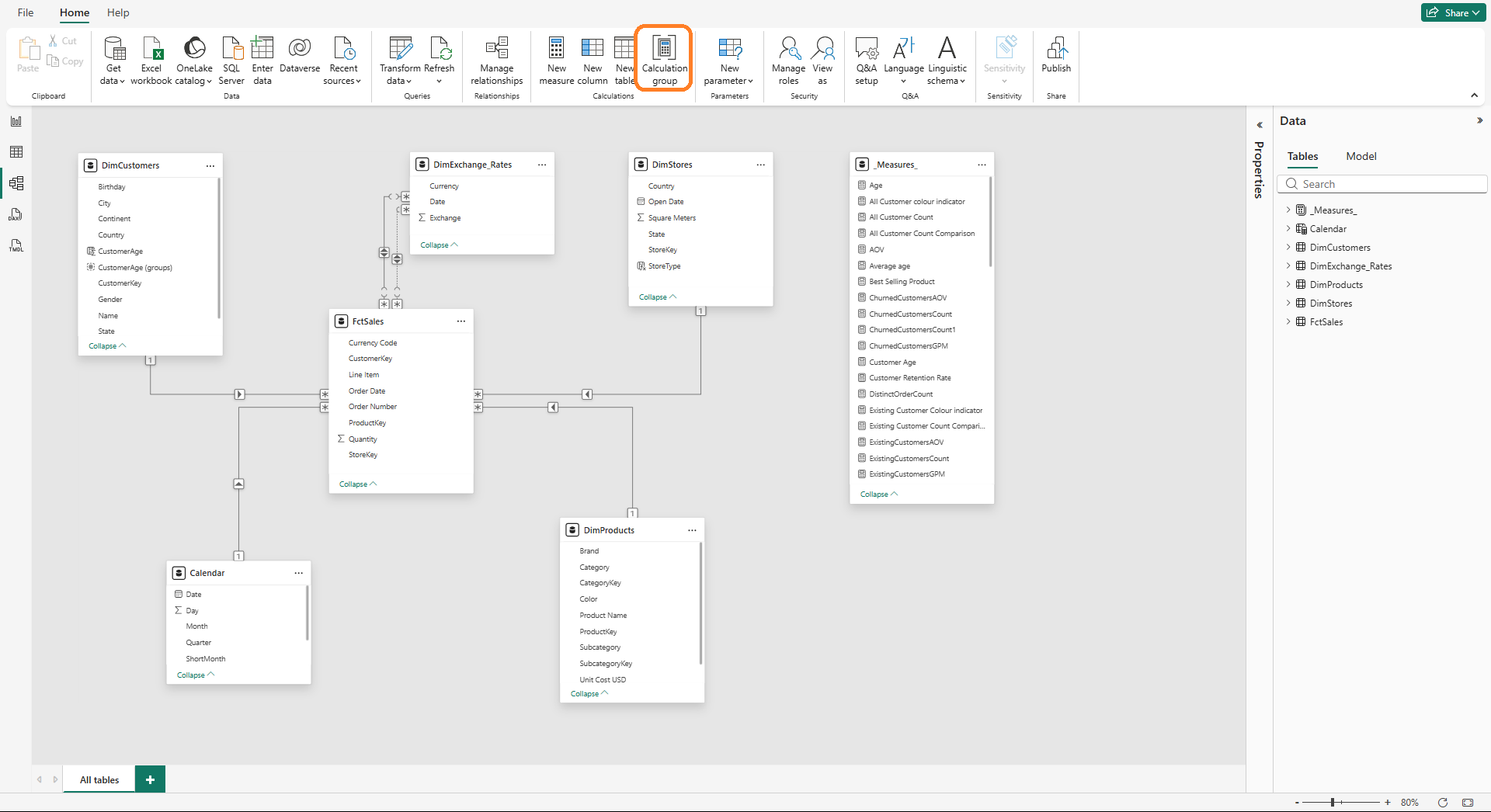
How to create it?
1. Navigate to Model View, find the Calculation group button in the ribbon and click on it.
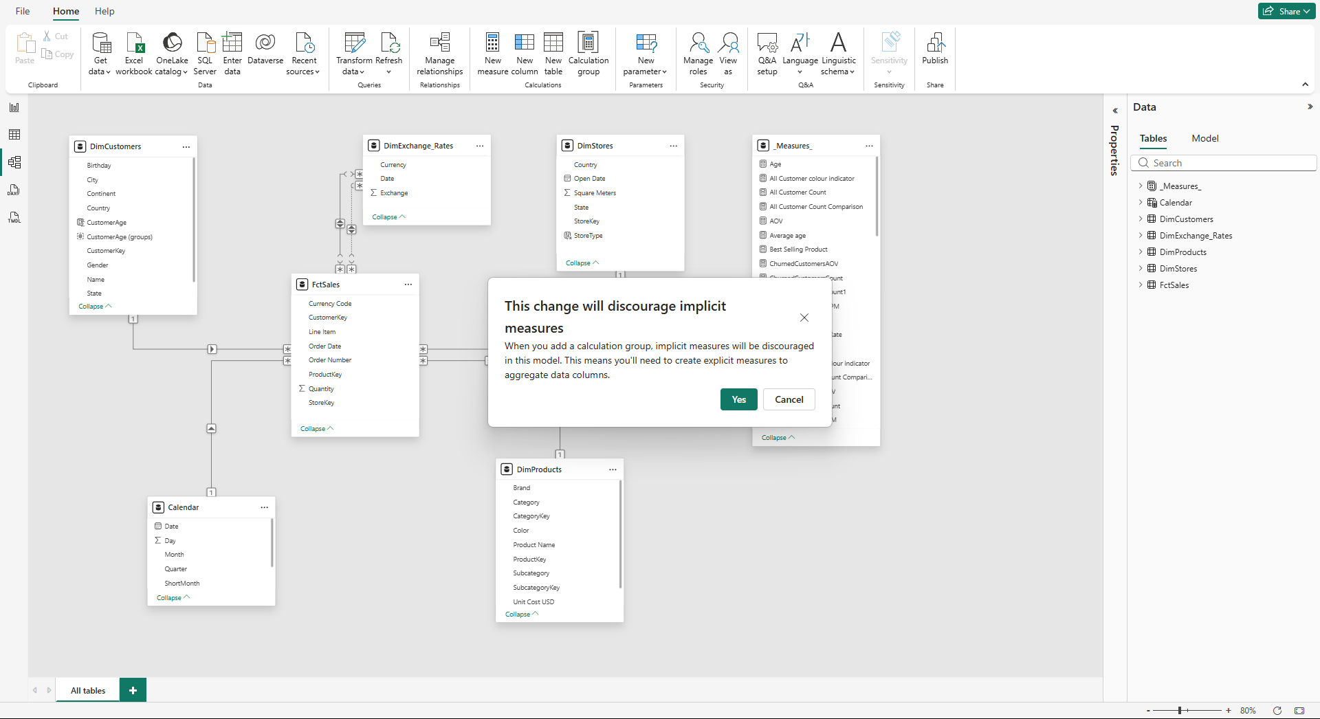
2. You will get a message about discouraging the implicit measures, and that means that you have to create a new measure for each aggregation you want to use on your dashboard.
3. Create a new calculation and press Enter.
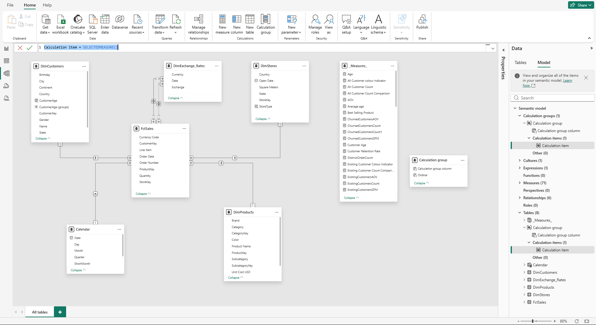
4. Go back to the Report View. You will see a new group appear in the same place on the right, where you have all your measures.
Now you can use it in your dashboard. One of the options is to use it as a slicer.
Code examples:
Year-to-Date (Time Intelligence):
Use the SELECTEDMEASURE() function as a placeholder, applying the same logic to any base measure (Sales, Profit, or Units).
YTD =
CALCULATE(
    SELECTEDMEASURE(),
    DATESYTD(’Date’[Date])
)
2. Activate Inactive Relationships:
Calculation groups can switch the active relationship in a model with USERELATIONSHIP() function. This is a good solution for analyzing data by different dates, such as Delivery Date versus Order Date, without creating duplicate measures.
Delivery Date =
CALCULATE(
    SELECTEDMEASURE(),
    USERELATIONSHIP(Sales[DeliveryDate], Date[Date])
)
3. Summary Statistics (Averages):
Instead of creating separate Average measures for every metric, you can create a calculation item that iterates over a table to provide summary statisticsfor a measure selected in the visual.
Average =
AVERAGEX(
    VALUES(’Product’[ProductName]),
    SELECTEDMEASURE()
)
4. Dynamic Format Strings:
Calculation groups can override the formatting of the base measure. For items like Year-over-Year Growth % it is critical because it should be displayed as a percentage even if the base measure is currency.
“0.00%;-0.00%;0.00%”You can use a SWITCH statement in the dynamic format string property to change the format based on the value size, for example, switching to “K” for thousands or “M” for millions:
SWITCH(
    TRUE(),
    SELECTEDMEASURE() >= 1000000, “#,0,,.0M”,
    SELECTEDMEASURE() >= 1000, “#,0,.0K”,
    “#.0”
)
Tooltips and Slicer Control:
Calculation groups can improve the interactivity of Custom Tooltips.
In a standard matrix with multiple measures (Orders, Quantity, Sales), hovering over a cell shows a generic tooltip.
Enable a calculation group on the tooltip page, and you can create a dynamic trend line that displays the trend for a measure that you hover over. The Calculation group, as a legend or axis in the tooltip visual, will filter the measure context based on the user’s hover point.
Selection expressions are also a good option when you select no item or multiple items in a slicer:
multipleOrEmptySelectionExpression: Defines what the report should show if you select more than one item (or none) in a slicer. Use this to display a message like “Please select only one calculation” or to default to a “Current” value.
noSelectionExpression: If nothing is selected in a currency or time slicer, the report defaults to a standard view (like USD or Current Year) rather than showing blank results.
The Order of Application:
When a model contains multiple calculation groups (one for Time Intelligence and one for Currency Conversion), the order is critical. Precedence property controls that.
Precedence Rules:
Groups with higher precedence values are applied first.
The system creates a nested structure, where the logic of the higher precedence group replaces the
SELECTEDMEASURE()placeholder of the lower precedence group.
Example:
In a scenario with both YTD calculation and Currency Conversion, Time Intelligence is set to a higher rank (200) than Currency Conversion (100). YTD total is calculated first, and then the final result is converted to the target currency.
If the order were reversed, the currency conversion might happen on a daily basis, leading to errors when summed over the YTD period.
User Defined Functions (UDFs):
You can combine User Defined Functions (UDFs) with calculation groups to reduce code volume. In some scenarios with many inactive relationships, you can define a dynamic UDF that takes a measure and a column as parameters to activate a relationship via USERELATIONSHIP().
Instead of writing the same CALCULATE logic in every calculation item, call the UDF within the calculation group items. A few calculation items will manage dozens of relationship-measure combinations.
Performance and Model Efficiency:
You might think that adding layers of logic might slow down a report, but calculation groups improve performance. By replacing hundreds of separate measures with a few shared logic patterns, the engine has less metadata to manage.
Improvements:
Smaller Model Size: Fewer metadata objects lead to a better model performance.
Cache Usage: The engine can reuse calculations across different visuals, reducing the CPU load.
Metadata Load: Faster initial loading times for report visuals, as there are fewer individual measures to resolve.
You have to be cautious not to overcomplicate DAX within calculation items, as complex logic or excessive items (dozens in a single group) can impact rendering speed.
Common Pitfalls:
1. Implicit Measures Disabled: You should create explicit DAX measures for everything, which can be a thing, but with the help of LLM, that is not a big issue.
2. Variant Data Type: Upon adding a calculation group, Power BI reports use the variant data type for measures. This can cause issues with dynamic titles or certain visuals that expect a strict numeric type. Wrapping expressions in the FORMAT() function is a workaround.
3. Non-Numeric Measures: If you apply a calculation item (like YTD) to a non-numeric measure (like a text-based dynamic title), it will result in an error. Use ISNUMERIC(SELECTEDMEASURE()) within their calculation items to skip non-numeric operations and prevent report crashes.
4. Subtotals in Matrices: Calculation groups can interfere with subtotals, as Power BI cannot sum different calculation types (like Current and YTD) in the same column.
Best Practices:
Keep Base Measures Simple: Apply calculation items to simple, single-measure expressions rather than already complex, nested formulas.
Clear and Descriptive Naming: Use everyday language for calculation items (“Year to Date” instead of “YTD_Calc_01”) to make slicers intuitive.
One Purpose Per Group: Separate logic into focused groups, for example, one for “Time Intelligence” and another for “Currency”, to keep the interface clean and precedence manageable.
Get the Basics First: You should master a single group before attempting to use multiple interacting groups with complex precedence settings.
Testing: Use tools like DAX Studio or Performance Analyzer to verify results and check the impact on query speed.
Calculation Groups vs. Other Features:
There are other dynamic features in Power BI, and it is important to know when to use each:
Field Parameters: Best used for switching between different metrics ( Sales vs. Profit) or different dimensions (Category vs. Region). While they can overlap in some measure in switching scenarios, calculation groups are superior for applying the same logic to many measures.
Visual Calculations: These are local to a chart and excellent for quick notes or one-off visuals. Calculation groups provide reusable logic that can be shared across all pages.
Calculation groups solve the problem of excessive measure with reusable logic. SELECTEDMEASURE() placeholder transforms a single formula to an unlimited number of measures across the entire data model.
For this approach you need to write explicit DAX measures, but the benefits will outweigh that: smaller model sizes, faster maintenance, consistent calculations.
As used for time intelligence, complex currency conversion, or advanced dynamic formatting, calculation groups are an essential tool for you when aim to build scalable and efficient enterprise-level reports.
💡Subscribe to learn more advanced DAX techniques that simplify and speed-up you work.
What is the most frustrating part of managing your current Power BI reports?
Let me know in the comments. 👇
Calculation groups are a game-changer